Chapter 6 Understanding additive traits
6.1 Introduction
Additive genetic variation is the only heritable variance component, and as such, the most important to selection.
6.2 Simulating a population to explore additive traits
pop_haps <- quickHaplo(nInd = 1000,
                       nChr = 1,
                       segSites = 100,
                       genLen = 1,
                       ploidy = 2L,
                       inbred = FALSE)

SP <- SimParam$new(pop_haps)

SP$addTraitA(nQtlPerChr = 10, # number of QTL for trait
             mean = 100, # mean genetic value of the trait
             var = 10, # variance of trait
             corA = NULL, # matrix of correlations between additive effects
             gamma = FALSE,  # to use a gamma distribution in place of a normal distribution
             shape = 1, # shape parameter for gamma distribution only
             force = FALSE) # keep false until this is understood!

SP$setVarE(h2 = 0.5, # narrow sense heritability
           H2 = NULL, # broad sense heritability
           varE = NULL) # error variance

pop_0 <- newPop(pop_haps,
                simParam = SP)
6.3 Breeding, genetic, and phenotypic value
In creating an additive trait and defining an environmental variance, AlphaSimR assigns a phenotypic value to each individual. The phenotypic value is based in part on the genotype of each individual at the designated quantitative trait loci (QTL), and part on the environmental variance parameter set when we defined narrow sense heritability as 0.5. In quantitative genetic terms, the phenotypes were simulated through a combination of non-random genetic and random environmental effects. Given our trait is completely additive, genetic effects are synonymous with additive effects in this particular case.
In the real world we would only know the phenotypes. It would then be our job to partition the phenotypic variance into additive and environmental effects at the very least. In fact, this is what we will be doing in Chapters 2-6. For the purpose of this exercise, we can take advantage of the fact that this is a simulation and ‘call’ our effects directly. The following code calls individual phenotypic, genetic, and breeding values, and arranges them in a data frame.
pv_gram <- pheno(pop_0)
gv_gram <- gv(pop_0)
bv_gram <- bv(pop_0) + mean(gv(pop_0))
pv_norm <- pheno(pop_0) - mean(pheno(pop_0))
gv_norm <- gv(pop_0) - mean(gv(pop_0))
bv_norm <- bv(pop_0)

ind_vals <- data.frame(pv_gram, gv_gram, bv_gram, pv_norm, gv_norm, bv_norm)
head(round(ind_vals, 2))
## pv_gram gv_gram bv_gram pv_norm gv_norm bv_norm
## 1 99.40 94.01 94.01 -0.58 -5.99 -5.99
## 2 97.83 101.85 101.85 -2.16 1.85 1.85
## 3 104.54 102.55 102.55 4.56 2.55 2.55
## 4 103.95 103.88 103.88 3.96 3.88 3.88
## 5 95.62 94.64 94.64 -4.36 -5.36 -5.36
## 6 96.44 99.25 99.25 -3.54 -0.75 -0.75From the first few lines it seems genetic values and breeding values are the same. This makes sense since our simulation includes neither dominance, epistatic, or GxE effects. As such, genetic values equal breeding values which in turn derived from the additive component of phenotypic variance. Given that the estimation of breeding values is a principle theme throughout later chapters further details are limited here. However, it should be understood that the called breeding values are ‘true’ breeding values and not derivations arrived at through phenotypic analysis. True breeding values, of course, are vitally important to the assessment of the breeding value estimates arrived through simulation.
Through a plot of individual breeding values as a function of phenotypic values we can visualize some fundamental concepts to genetics and breeding.
plot_gram <- ind_vals %>% ggplot(aes(x = pv_gram, y = bv_gram)) +
                                     geom_point() +
                                     geom_smooth(method='lm', formula= y ~ x)

plot_norm <- ind_vals %>% ggplot(aes(x = pv_norm, y = bv_norm)) +
                                     geom_point() +
                                     geom_smooth(method='lm', formula= y ~ x)

grid.arrange(plot_gram, plot_norm, ncol = 2)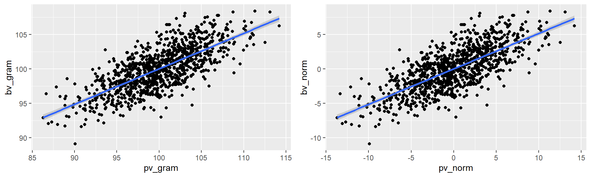
gram_mod <- lm(bv_gram ~ pv_gram, data = ind_vals)
norm_mod <- lm(bv_norm ~ pv_norm, data = ind_vals)

y_int <- c(coef(gram_mod)[1], coef(norm_mod)[1])
slope <- c(coef(gram_mod)[2], coef(norm_mod)[2])
herit <- c(cov(ind_vals$pv_gram, ind_vals$bv_gram) / var(ind_vals$pv_gram),
           cov(ind_vals$pv_norm, ind_vals$bv_norm) / var(ind_vals$pv_norm))
accur <- c(cor(ind_vals$pv_gram, ind_vals$bv_gram),
           cor(ind_vals$pv_norm, ind_vals$bv_norm))

pop_stats <- data.frame(y_int, slope, herit, accur)
round(pop_stats, 3)
## y_int slope herit accur
## pv_gram 48.423 0.516 0.516 0.73
## pv_norm 0.000 0.516 0.516 0.736.4 Heritability of additive traits
We just demonstrated that the phenotype of an additive trait is derived from two components, a nonrandom additive component and a random environmental component. We will momentarily delve deeper into the additive component, but take a moment here to further explore random environmental effects. In some animal breeding texts you will hear environmental effects described as ‘nuisance’ effects. This is an apt description given the definition of nuisance as, “a circumstance causing inconvenience or annoyance”. The reason environmental effects can become a nuisance stems from the fact that unlike additive effects that are correlative to genotypes, environmental effects are random.
The exploration of random variables is frequently performed using Monte Carlo simulations. As you might expect, R has a number of tools to support the development and analysis of Monte Carlo simulations. As a general guide, a function under the influence of a random variable is first written and the repeated using a function from the apply family. The following code creates a function called h2_MC from the population simulation script employed at the beginning of the chapter. The function takes a single argument, heritability, and returns the calculated heritability and accuracy of the simulated population. Each time the script is run all individuals are assigned a phenotype that is in turn based on a genotype-dependent breeding value and a random environmental effect. In this case, the random environmental effect is the objective of the Monte Carlo simulation.
h2_MC <- function(h2){
         pop_haps <- quickHaplo(nInd = 10, nChr = 1, segSites = 100, genLen = 1, ploidy = 2L, inbred = FALSE)
         SP = SimParam$new(pop_haps)
         SP$addTraitA(nQtlPerChr = 10, mean = 100, var = 10, corA = NULL, gamma = FALSE, shape = 1, force = FALSE)
         SP$setVarE(h2 = h2, H2 = NULL, varE = NULL)
         pop_0 <- newPop(pop_haps, simParam = SP)
         return(list(cov(pop_0@pheno, pop_0@gv) / var(pop_0@pheno), cor(pop_0@pheno, pop_0@gv)))}
After creating the function we can now use the lapply function to simulate population development as many times as we want. The following code simulates one thousand populations with a parameter heritability setting of 0.5, and returns the calculated heritability and accuracy. Results are returned as nested list items and then converted into a data frame for plotting as histograms. Histograms of both heritability and accuracy are produced.
mc_results <- lapply(rep(0.5, 1000), h2_MC)
h2 <- unlist(sapply(mc_results, function(x) x[1]))
r2 <- unlist(sapply(mc_results, function(x) x[2]))
mc_df <- data.frame(h2, r2)

plot_h2 <- mc_df %>% ggplot() +
                     geom_histogram(aes(x = h2),
                                    binwidth = 0.05,
                                    color = 'black',
                                    fill = 'blue',
                                    alpha = 0.5) +
                     xlim(c(0, 1))
plot_r2 <- mc_df %>% ggplot() +
                     geom_histogram(aes(x = r2),
                                    binwidth = 0.05,
                                    color = 'black',
                                    fill = "light blue",
                                    alpha = 0.5) +
                     xlim(c(0, 1))

grid.arrange(plot_h2, plot_r2, nrow = 1)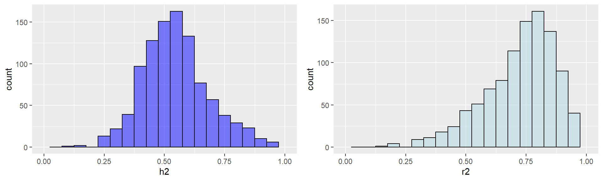
Through the Monte Carlo simulation we find more variation than we might expect. In terms of heritability, a fairly normal distribution centered on, or near, the simulation parameter of 0.5 is noted. Deviations from 0.5 are not reflective of additive effects accounting for more or less than 50% of the phenotype, but rather correlations between additive and environmental effects. For example, if smaller fish are randomly assigned larger environmental component and larger fish smaller environmental effects, observed heritability decreases. If larger fish are randomly assigned larger environmental effects and smaller fish smaller environmental effects, heritability increases. It is important to note that in this case such correlations are arising randomly and not systematically. Evidence for randomness is in the heritability distribution itself. If the center of our distribution was significantly different from 0.5, we would have to consider why our simulation is resulting in underlying gene x environment effects.
If we now turn our attention to our distribution of prediction accuracy. We can see that rather than being normal, our distribution is skewed to the right and has a long left hand tail. In fact, rather than being normal the resulting accuracies resemble a beta distribution. This is quite normal for random variables with finite intervals such as R2 values that should always be between 0 and 1. It is only strange in that we don’t see the same for heritability when it increases towards 1, the theoretical limit. Heritability, however, is not mathematically constrained to this interval. In our particular case, heritability can exceed values of 1 by ‘unknowingly’ including GE effects in the numerator and not in the denominator.
It is also important to understand the relationship between heritability and accuracy. Accuracy, of course, is a measure of the degree to which we can predict phenotype from a breeding value. Due to its random nature, environmental variation itself reduces accuracy of